Magnetic Vortex-Spinwave Scattering Functions
G. M. Wysin, Kansas State University, Spring 2000.
Magnetic Vortices and Spinwaves
 These are data showing the spin-wave-functions of the spinwaves
in the presence of an in-plane magnetic vortex in a two-dimensional magnet.
The spinwave modes were found by a relaxation method, which gives
both the wavefunctions and frequencies of some of the lowest modes.
We considered ferromagnetic and antiferromagnetic models.
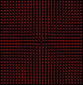
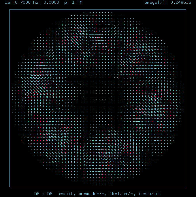
A vortex in a ferromagnet is shown to the right.
These are data showing the spin-wave-functions of the spinwaves
in the presence of an in-plane magnetic vortex in a two-dimensional magnet.
The spinwave modes were found by a relaxation method, which gives
both the wavefunctions and frequencies of some of the lowest modes.
We considered ferromagnetic and antiferromagnetic models.
A vortex in a ferromagnet is shown to the right.
Easy-Plane Magnetic Model
The nearest-neighbor Hamiltonian has easy-plane anisotropy parameter
lambda, in a form
Hn,m = J * Sn . Sm
where the Sn are three-component spins and J is a diagonal matrix:
        1   0   0

 J  =   0   1   0

        0   0  lambda
We consider a square lattice of spins, with a circular boundary
at radius R, and 0 <= lambda < lambda_c, where lambda_c = 0.7034
is the critical anisotropy parameter. For this anisotropy range,
the vortex configuration is purely in the xy-plane (in-plane vortex).
Fixed boundary conditions were used.
Spinwave Modes
The modes are labeled by a principle quantum number 'n' and azimuthal
quantum number 'm', and represent the possible forms of oscillation
of the spin field, on top of the original vortex structure.
omega is the oscillation frequency. The quantum numbers are
the numbers of nodal lines in the radial and azimuthal directions,
respectively.
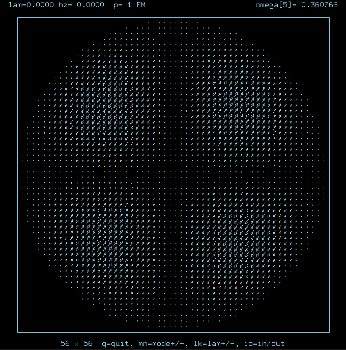
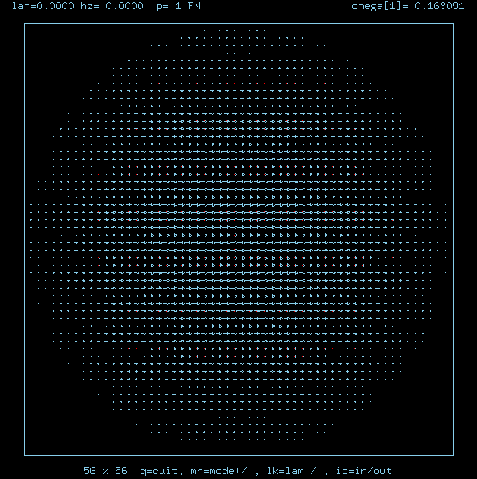
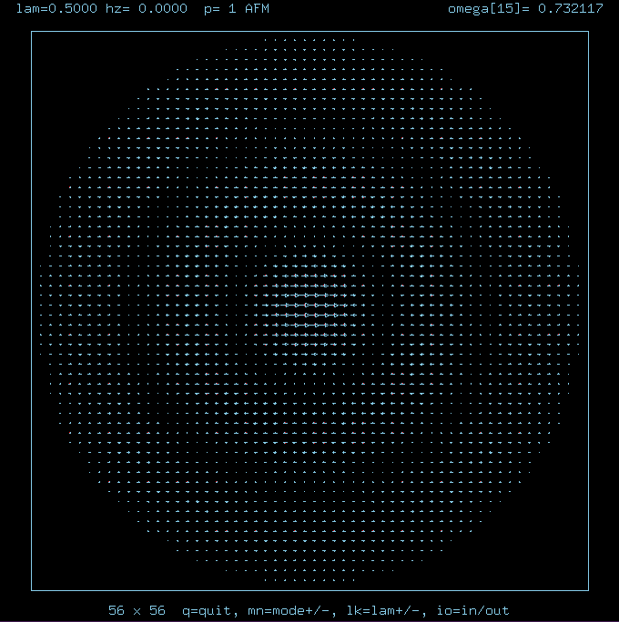
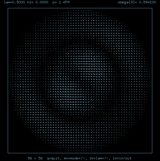
On the mode diagrams below, blue arrows represent the magnitude (arrow length)
and phase (arrow direction) of the oscillations of in-plane (xy) spin components.
Red arrows represent the magnitude (arrow length) and phase (arrow direction)
of the out-of-plane (z) spin components.
Scattering and S-matrix
The S-matrix is derived from fitting the wavefunctions to a
sum of incoming plus outgoing waves, with amplitude of the
outgoing waves relative to the incoming ones being called 'S'.
The in-plane part of the wavefunctions was fit to a form like
Psi = A [ Jm(kr) + rhom(k) Ym(kr) ]
where Jm and Ym are Bessel functions, and A and
rhom(k) are fitting constants. 'k' is the wavevector
for a spinwave, which can be derived from the spinwave dispersion
relation because we know the spinwave frequency. Sm(k)
is then derived from rhom(k), by a simple formula,
Sm(k) = [1 - i rhom(k) ]/[1 + i rhom(k) ]
Below we show some plots of the results obtained for rhom(k),
for only the acoustic branch spinwaves (not for the local mode of
the AFM model, which is from the optical branch).
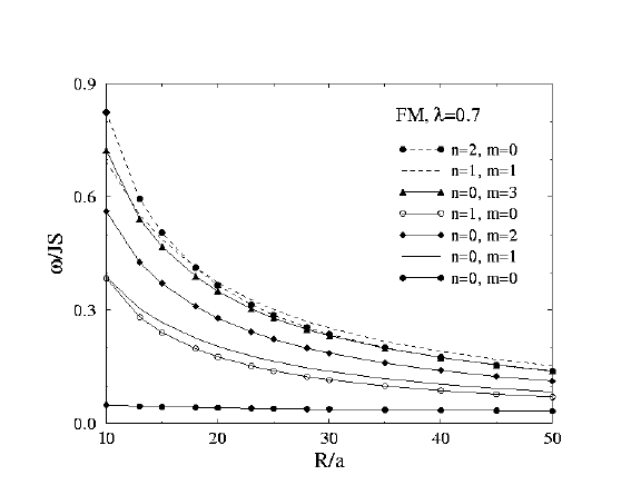
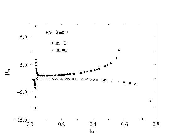
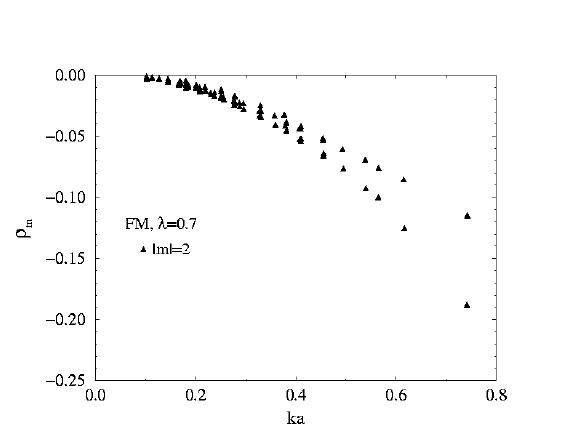
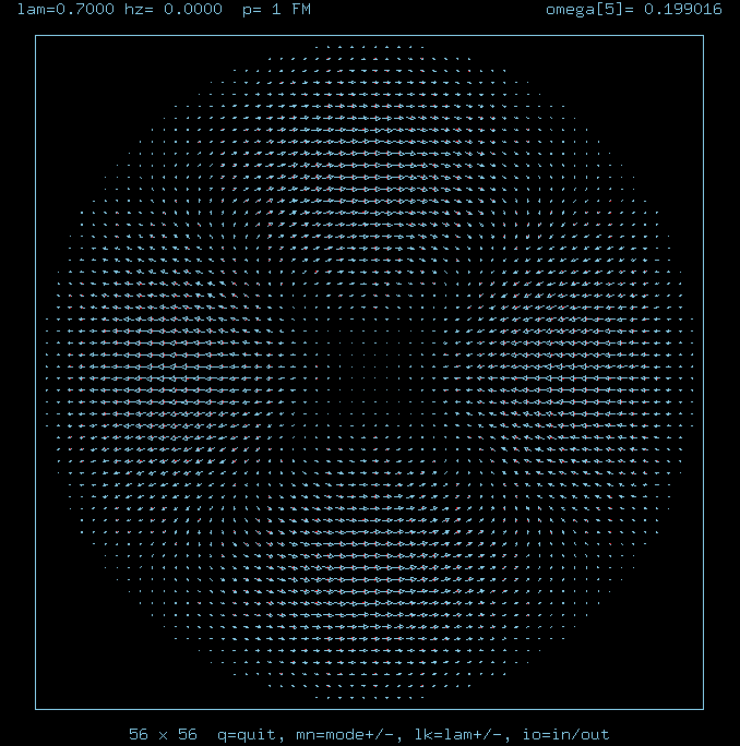
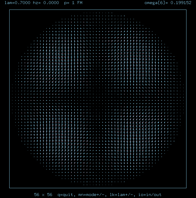
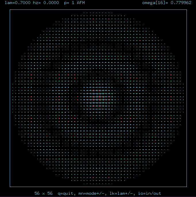
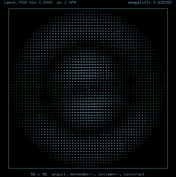
Ferromagnet at lambda=0.7
This is anisotropy parameter just below the critical value of lambda_c=0.7034,
above which the static vortex would possess an out-of-easy-plane component.
Here, the lowest mode, n=0, m=0, has frequency nearly independent of system
radius. This mode is the vortex instability mode, and is quite local in
out-of-plane oscillations, but extended in in-plane oscillations.
Note also the interesting singularities in the scattering for m=0,
but smoother behavior at m=1, 2.
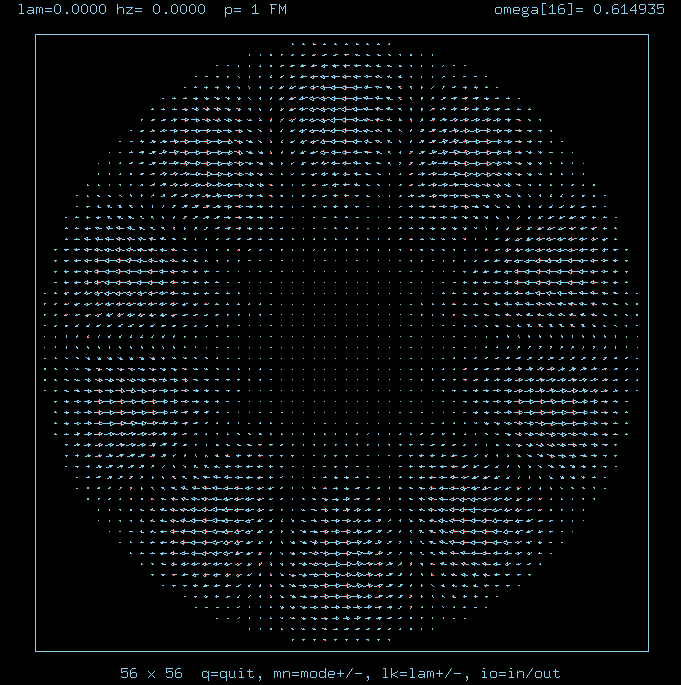
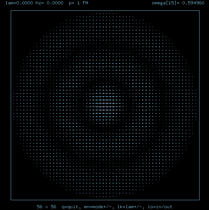
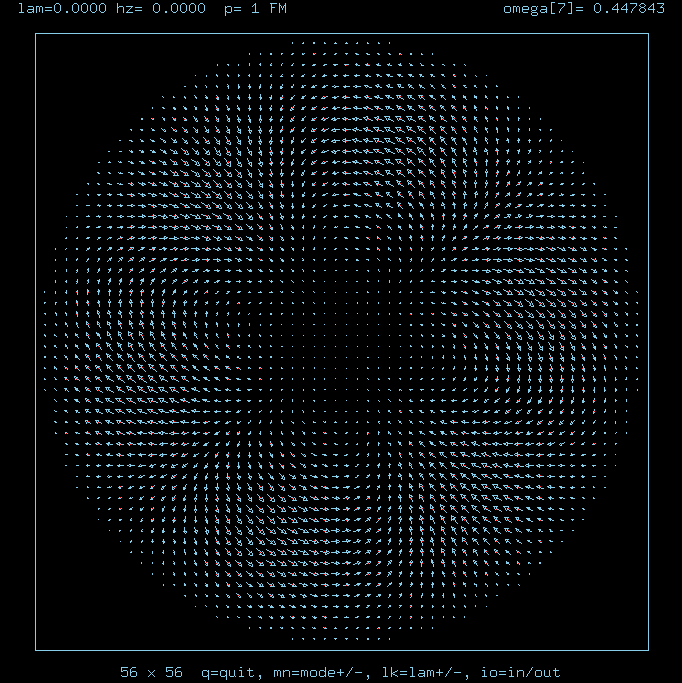
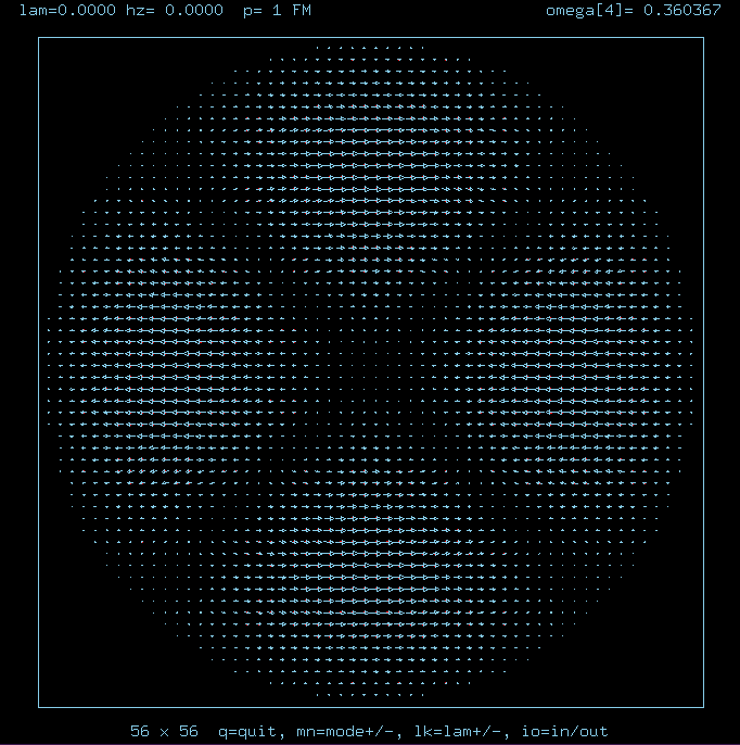
Vortex-Spinwave
Scattering Modes for
Ferromagnet
R=28, lambda=0.7
n=2, m=0,
n=1, m=1,
n=0, m=3,
n=1, m=0,
n=0, m=2,
n=0, m=2,
(m=2 states not exactly degenerate, due to lattice)
n=0, m=1,
(translational mode)
n=0, m=0,
(quasi-local mode or vortex-instability mode)
|
Spinwave frequencies vs. system radius R, Ferromagnet, lambda=0.7
|
Scattering Rates for
Ferromagnet
lambda=0.7
m=0, 1
|
|
Scattering Rates for
Ferromagnet
lambda=0.7
m=2
|
|
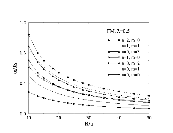
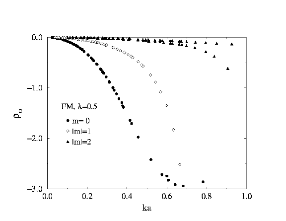
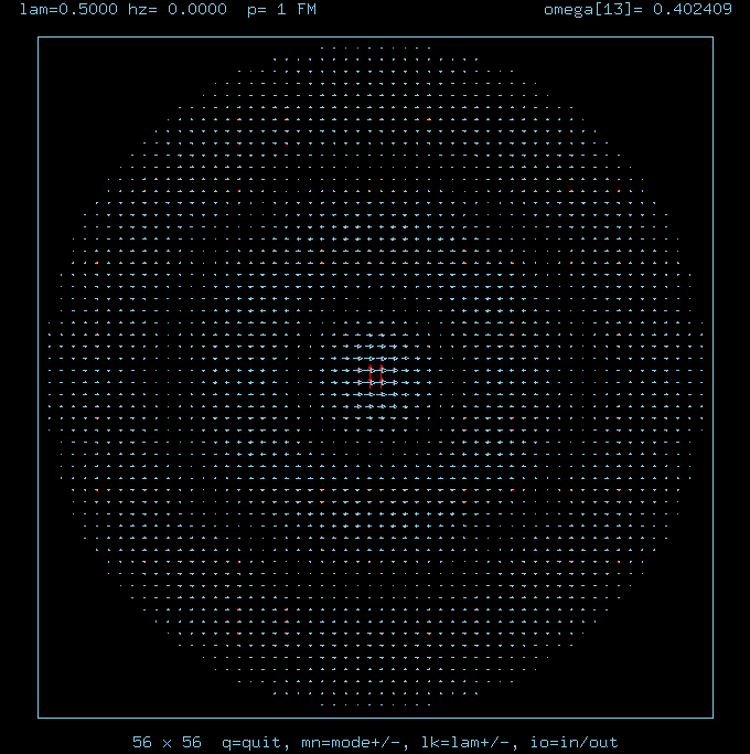
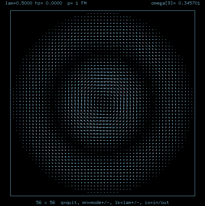
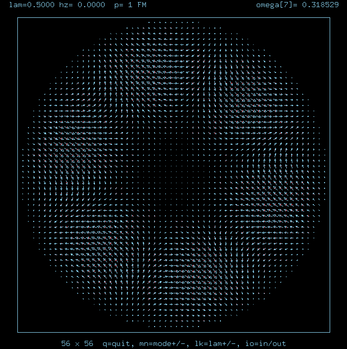
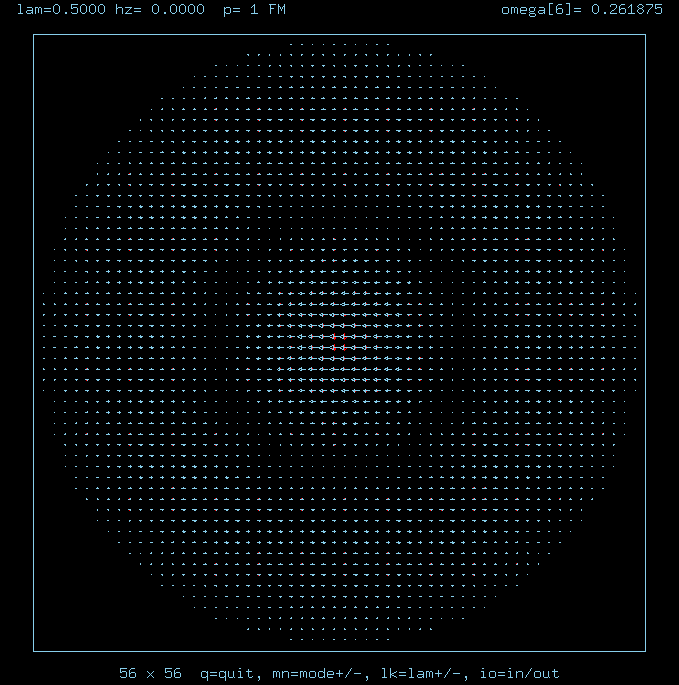
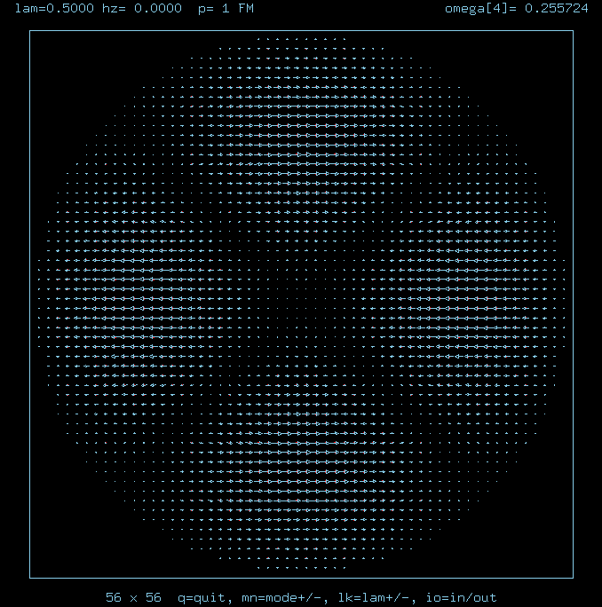
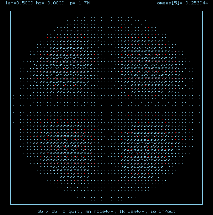
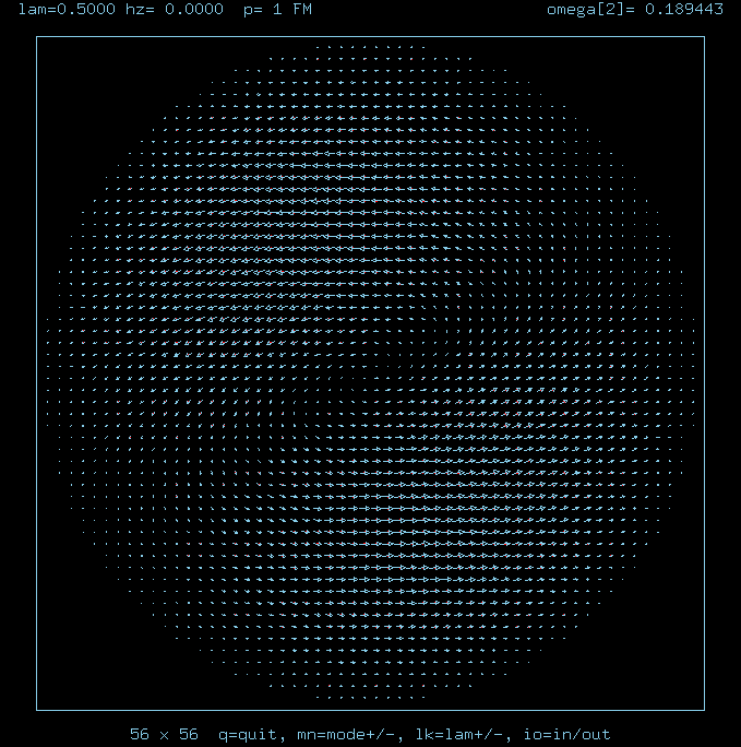
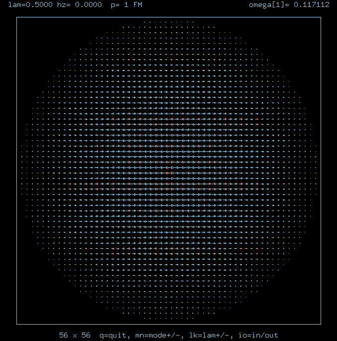
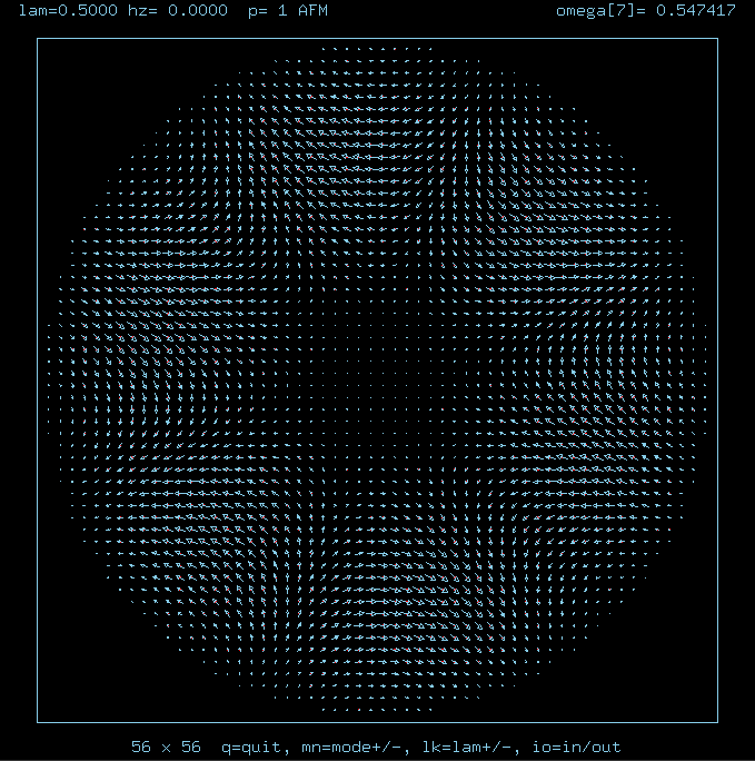
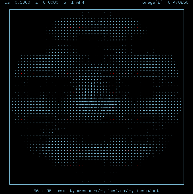
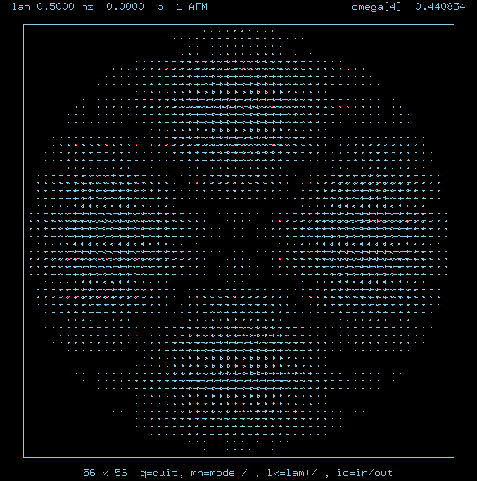
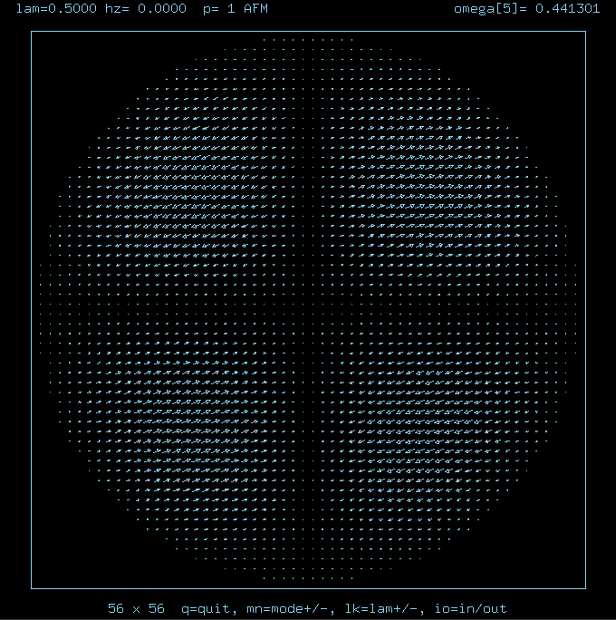
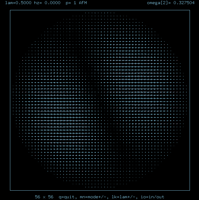
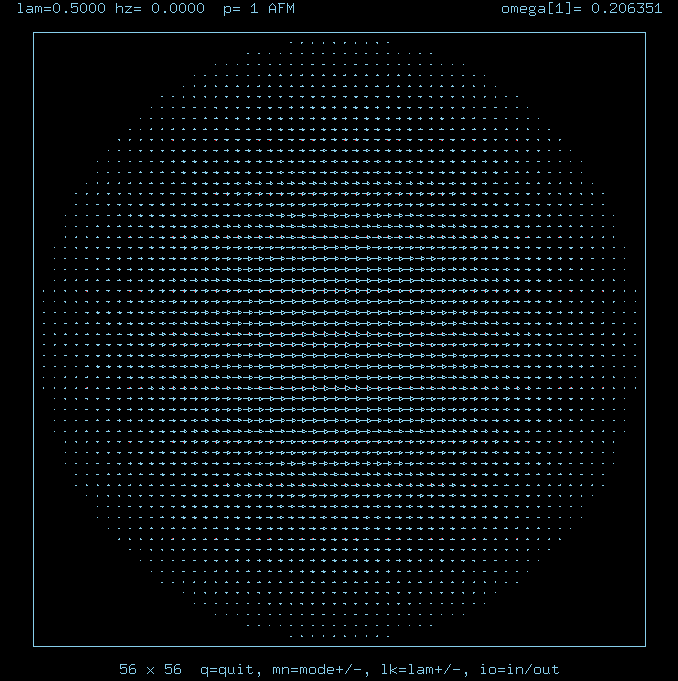
Ferromagnet at lambda=0.5
Farther from the critical anisotropy. The n=0, m=0 mode now has
considerable frequency change with system radius. Scattering at m=0
is smoother, no singularities appeared over the range of k studied.
Vortex-Spinwave
Scattering Modes for
Ferromagnet
R=28, lambda=0.5
n=2, m=0,
n=1, m=1,
n=0, m=3,
n=1, m=0,
n=0, m=2,
n=0, m=2,
(m=2 states not exactly degenerate, due to lattice)
n=0, m=1,
(translational mode)
n=0, m=0,
(quasi-local mode or vortex-instability mode)
|
Spinwave frequencies vs. system radius R, Ferromagnet, lambda=0.5
|
Scattering Rates for
Ferromagnet
lambda=0.5
m=0, 1, 2
|
|
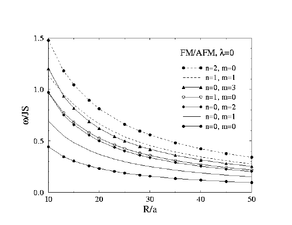
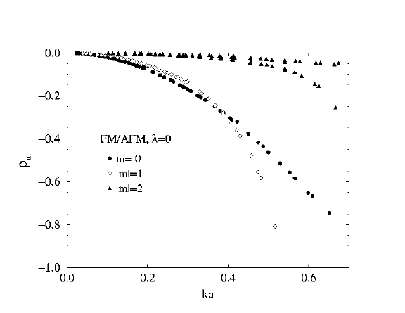
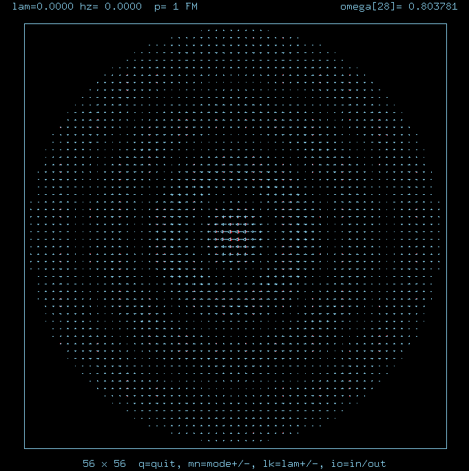
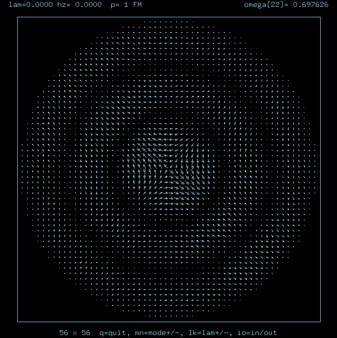
FM or AFM at lambda=0
At this anisotropy value, the eigenvalue problem for the spinwaves is
the same for FM and AFM models, so they have identical spinwave frequencies
and wavefunctions. As a result, even the scattering rates rhom(k)
are the same.
Also note: the n=0, m=0 mode here evolves into the vortex instability
mode as lambda approaches lambda_c for the FM model. However, this mode
does nothing interesting as lambda approaches lambda_c for the AFM model.
The truly local mode of the AFM model actually comes down from a higher
frequency mode taken out of the optical spinwave branch. See the results
for lambda=0.7 for AFM model, below.
|
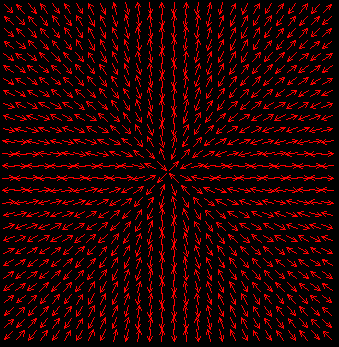
An in-plane vortex in an antiferromagnet
|
Vortex-Spinwave
Scattering Modes for
Ferromagnet
or Antiferromagnet
R=28, lambda=0.0
(These have identical spectra.)
n=3, m=0,
n=2, m=1,
n=0, m=5,
n=2, m=0,
n=1, m=1,
n=0, m=3,
n=1, m=0,
n=0, m=2,
n=0, m=2,
(m=2 states not exactly degenerate, due to lattice)
n=0, m=1,
(translational mode)
n=0, m=0,
(lowest mode --> FM quasi-local mode)
|
Spinwave frequencies vs. system radius R, Ferromanget or Antiferromagnet, lambda=0.0
|
Scattering Rates for
Ferromagnet
or Antiferromagnet
lambda=0.0
m=0, 1, 2
|
|
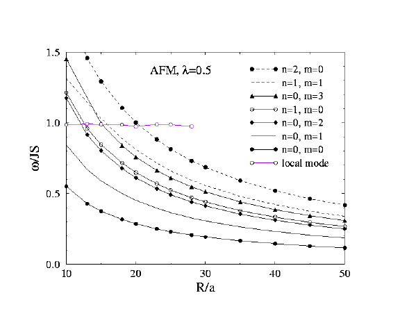
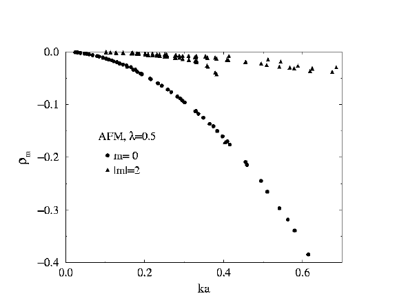
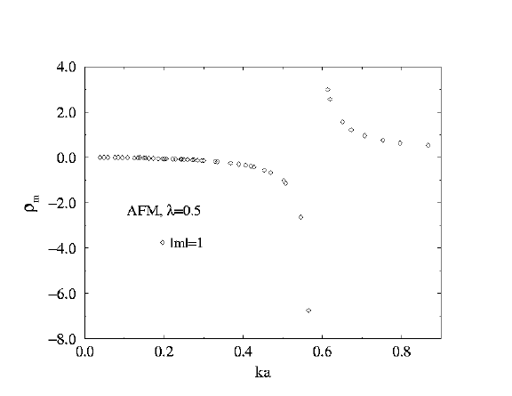
Antiferromagnet at lambda=0.5
Check out the local mode that appears near omega/JS = 1, independently
of the system radius (purple curve on figure). The other modes tend to
have frequencies diminishing as 1/R. The red arrows
displayed in the wavefunction for this mode show that oscillations
of the out-of-easy-plane components are becoming important.
The mode here is actually a mixture of m=0 and m=2 components.
Vortex-Spinwave
Scattering Modes for
AntiFerromagnet
R=28, lambda=0.5
n=0, m=0,
(truly local mode or vortex-instability mode, optical branch)
n=2, m=0,
n=1, m=1,
n=0, m=3,
n=1, m=0,
n=0, m=2,
n=0, m=2,
(m=2 states not exactly degenerate, due to lattice)
n=0, m=1,
(translational mode)
n=0, m=0,
(lowest mode, extended, acoustic branch)
|
Spinwave frequencies vs. system radius R, Antiferromagnet, lambda=0.5
|
Scattering Rates for
AntiFerromagnet
lambda=0.5
m=0, 2
|
|
Scattering Rates for
AntiFerromagnet
lambda=0.5
m=1
|
|
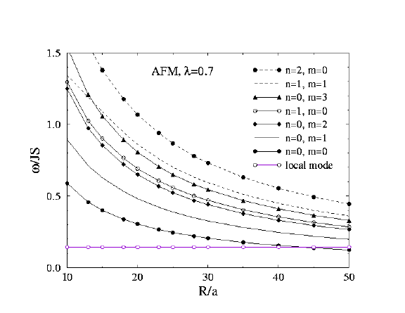
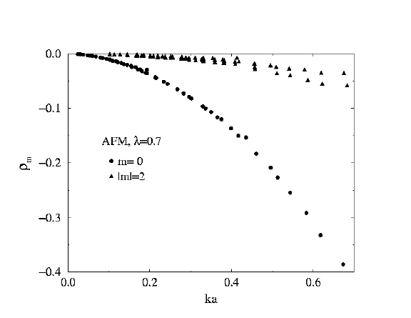
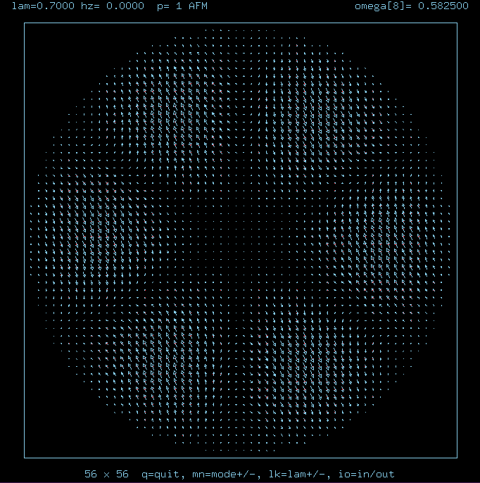
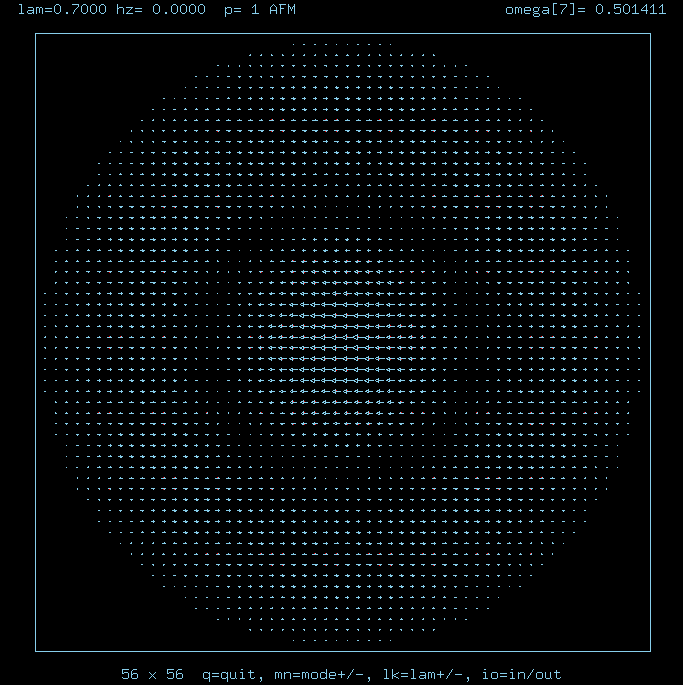
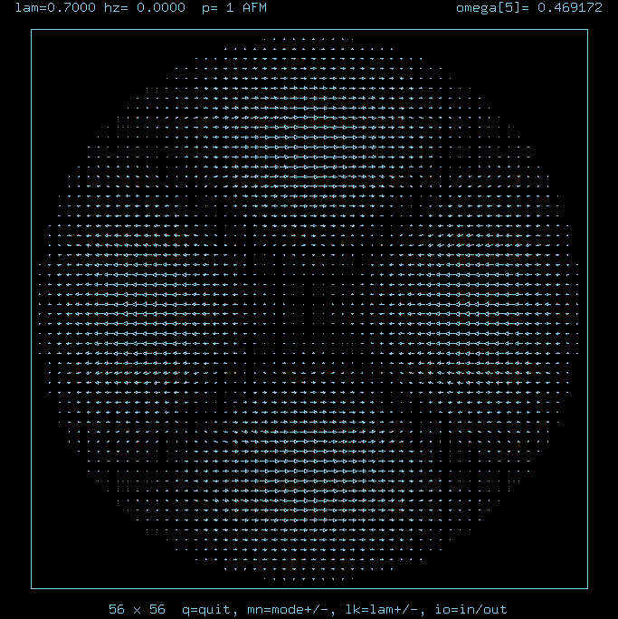
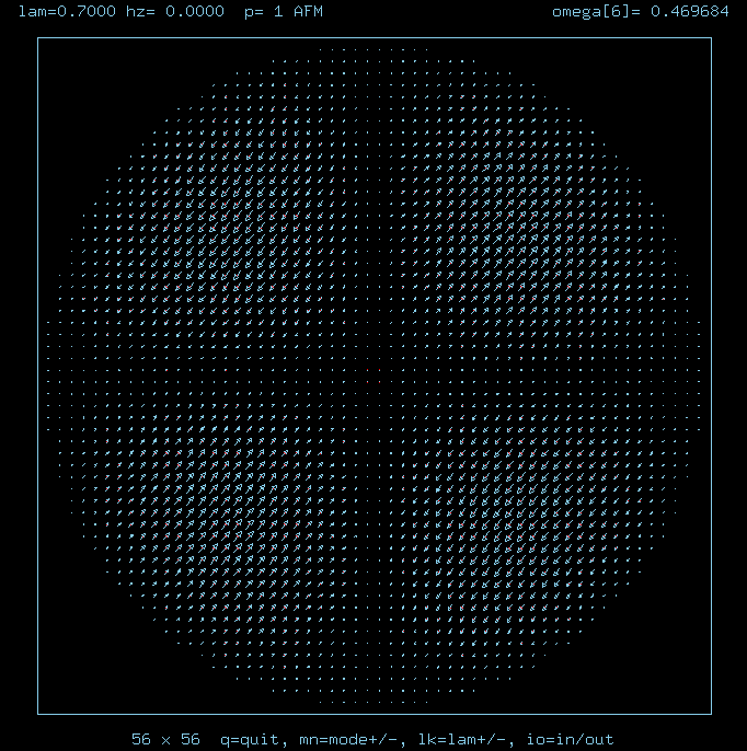
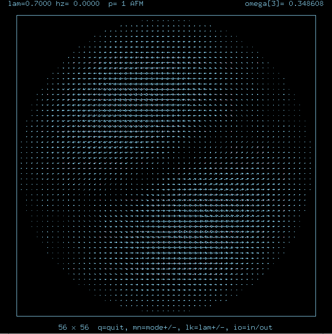
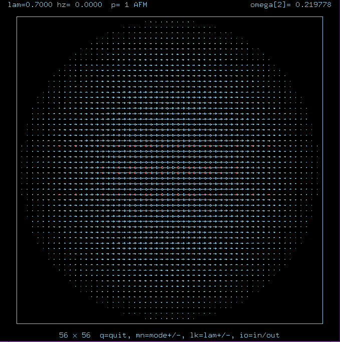
Antiferromagnet at lambda=0.7
Now the local mode has moved down near near omega/JS = 0.143, independently
of the system radius (purple curve on figure). The other modes still tend to
have frequencies diminishing as 1/R. The stronger red arrows
displayed in the wavefunction for this mode (compared to how it looked
at lambda=0.5) show that oscillations
of the out-of-easy-plane components dominate in this mode. Thus it
is also associated with how this in-plane vortex tries to become an
out-of-plane vortex as lambda approaches lambda_c=0.7034 .
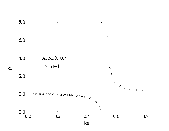
Both here and at lambda=0.5 a singularity appears in the m=1
scattering at fairly large wavevector.
Vortex-Spinwave
Scattering Modes for
AntiFerromagnet
R=28, lambda=0.7
n=2, m=0,
n=1, m=1,
n=0, m=3,
n=1, m=0,
n=0, m=2,
n=0, m=2,
(m=2 states not exactly degenerate, due to lattice)
n=0, m=1,
(translational mode)
n=0, m=0,
(extended mode, acoustic branch)
n=0, m=0,
(truly local mode or vortex-instability mode, optical branch)
|
Spinwave frequencies vs. system radius R, Antiferromagnet, lambda=0.7
|
Scattering Rates for
AntiFerromagnet
lambda=0.7
m=0, 2
|
|
Scattering Rates for
AntiFerromagnet
lambda=0.7
m=1
|
|
Other Links At KSU
access since 99/02/09.
Last update: Thursday June 22 2000.
email to -->
wysin@phys.ksu.edu