In what follows we impose semiclassical quantization by considering the
operators  to be quantum operators, satisfying the
Heisenberg equations of motion:
to be quantum operators, satisfying the
Heisenberg equations of motion:
with the standard canonical commutators,
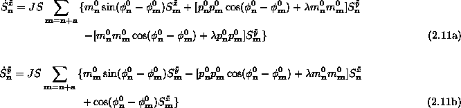
and its cyclic permutations. Because we are studying the small amplitude
deviations from the static vortex configuration, we need the equations of
motion linearized in  and
and  ,
with
,
with  . Doing so, we obtain
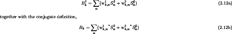
Now we look for eigenstates or normal modes, in the sense that we try to find
operators which are linear combinations of the  and
and
 operators, with a single-frequency time dependence.
Or, in quantum language, we look for creation and annihilation operators
operators, with a single-frequency time dependence.
Or, in quantum language, we look for creation and annihilation operators
 and
and  in which the Hamiltonian will be a sum of terms
in the simple diagonal form
in which the Hamiltonian will be a sum of terms
in the simple diagonal form  , where k is an index that
distinguishes the different modes making up a complete set. While the equations
are solved for finite systems, the usual momentum is not a good quantum number,
due to the lack of translational invariance. But the modes will be
distinguished by the effective wavelengths of the standing waves present, and
by the locations of nodes and antinodes in the wavefunctions or their
squares. In any case, we suppose the modes are ordered in some way, perhaps
from largest to smallest frequency, and notated by an index k. Some modes
may be energetically degenerate, in which case k must denote more than just
the frequency. It is clear that this type of problem will produce pairs of
conjugate modes,
, where k is an index that
distinguishes the different modes making up a complete set. While the equations
are solved for finite systems, the usual momentum is not a good quantum number,
due to the lack of translational invariance. But the modes will be
distinguished by the effective wavelengths of the standing waves present, and
by the locations of nodes and antinodes in the wavefunctions or their
squares. In any case, we suppose the modes are ordered in some way, perhaps
from largest to smallest frequency, and notated by an index k. Some modes
may be energetically degenerate, in which case k must denote more than just
the frequency. It is clear that this type of problem will produce pairs of
conjugate modes,  and
and  , and we suppose these unknown
operators are the linear combinations,
, and we suppose these unknown
operators are the linear combinations,
where the complex expansion coefficients  and
and
 are to be determined. (This being a linear problem,
there should be no confusion that
the superscripts ``1'' and ``2'' are not powers.) With the requirement of
are to be determined. (This being a linear problem,
there should be no confusion that
the superscripts ``1'' and ``2'' are not powers.) With the requirement of
 time dependence, where
  is the unknown
eigenfrequency to be determined,
is the unknown
eigenfrequency to be determined,  must satisfy
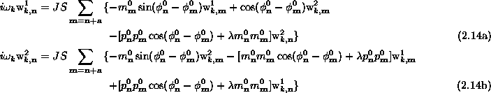
Using Eqs. (2.12) and (2.11) in Eq. (2.13) leads to the following matrix equation for the coefficients:
For numerical diagonalization, the lattice sites are numbered in some arbitrary
order, and then a vector can be formed out of the  and
and
 variables as
This will allow Eqs. (2.14) to be solved numerically for the eigenvalues
 and their respective eigenvectors, given in terms of the
coefficients
and their respective eigenvectors, given in terms of the
coefficients  and
and  . In this notation,
the matrix to be diagonalized is real, but not Hermitian.
. In this notation,
the matrix to be diagonalized is real, but not Hermitian.
Once we have the complete set of these normal modes and their eigenfrequencies, the Hamiltonian will be expressed in the diagonal form;
where  and
and  have equal frequencies, but with opposite
signs.
have equal frequencies, but with opposite
signs.